Hazard Emulator

Given a database of hazard events, the module climada.hazard.emulator provides tools to subsample events (or time series of events) from that event database. The module provides functionality to guard the subsampling, e.g., using bias-corrected statistics according to historical records in a specific georegion, or using calibrated statistics according to a climate scenario.

In more complex cases, the given event database is divided into a (smaller) set of observed hazard events and a (much larger) set of simulated hazard events. The database of observed events is used to statistically fit the frequency and intensity of events in a fixed georegion to (observed) climate indices. Then, given a hypothetical (future) time series of these climate indices (a “climate scenario”), a “hazard emulator” can draw random samples from the larger database of simulated hazard events that mimic the expected occurrence of events under the given climate scenario in the specified georegion.

The concept and algorithm as applied to tropical cyclones is originally due to Tobias Geiger (unpublished as of now) and has been generalized within this package by Thomas Vogt.

This notebook illustrates the functionality through the example of tropical cyclones in the eastern pacific under the RCP 2.6 climate scenario according to the MIROC5 global circulation model (GCM). However, the algorithm can be applied to arbitrary Hazard types given a suitable database of synthetic events.

Load hazard data

The database of hazard events for this tutorial is too large to be provided with it. Instructions on how to obtain or generate the data are provided in the last section of this tutorial. At this point, we load a precomputed Hazard object from a file that contains simulated tropical cyclone tracks for an RCP 2.6 climate scenario according to MIROC5. Note, however, that this module will work with any Hazard object, preferably containing a lot of events.

from climada.util.config import CONFIG
DEMO_DIR = CONFIG.local_data.demo.dir(create=False)
EMULATOR_DATA_DIR = DEMO_DIR.joinpath("emulator")

from climada.hazard import TropCyclone
hazard = TropCyclone.from_hdf5(EMULATOR_DATA_DIR.joinpath("hazard_360as_miroc_rcp26.hdf5"))

2021-03-24 17:46:31,484 - climada.hazard.base - INFO - Reading /home/tovogt/.climada/demo/data/emulator/hazard_360as_miroc_rcp26.hdf5

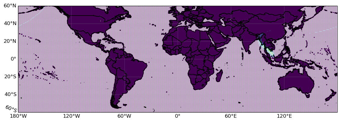
We quickly try to give an impression of what this particular Hazard object looks like. It contains hazard.size = 45300 tropical cyclone wind fields that are computed on a global set of centroids with 360 arc-seconds (0.1 degree) resolution onland and 1 degree resolution offshore. The physical effects onland are considered more important, the low-resolution information offshore is mostly relevant for plotting purposes:

import warnings; warnings.filterwarnings('ignore')
import matplotlib.pyplot as plt
import pyproj
plt.rcParams['figure.dpi'] = 120
hazard.centroids.geometry = hazard.centroids.geometry.to_crs(pyproj.CRS("EPSG:4326"))
hazard.centroids.plot(c=hazard.intensity[16637,:].toarray().ravel(), s=0.1);

<cartopy.mpl.geoaxes.GeoAxesSubplot at 0x7f74c8bb0a60>

Define the region of interest

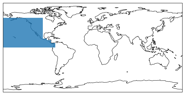
One basic feature of the climada.hazard.emulator module is the HazRegion class that not only defines the geographical region of interest for the statistics, but might also contain climatic information about the selected region, such as the cyclone (hurricane) season. For tropical cyclone hazards there already exists a derived class TCRegion that defines ocean basins and cyclone seasons.

import cartopy.crs as ccrs
import cartopy.feature as cfeature
from climada_petals.hazard.emulator.geo import TCRegion
# load Eastern Pacific basin, print season (months of year) and plot geometry
region = TCRegion(tc_basin="EP")
print(f"\nThe cyclone season in basin {region.tc_basin} spans "
      f"from month {region.season[0]} until month {region.season[1]}.\n")

ax = plt.gcf().add_axes([0, 0, 1, 1], projection=ccrs.PlateCarree())
ax.add_feature(cfeature.COASTLINE.with_scale('110m'), linewidth=0.75)
ax.add_geometries([region.shape], crs=ccrs.PlateCarree(), alpha=0.8);

The cyclone season in basin EP spans from month 7 until month 12.

<cartopy.mpl.feature_artist.FeatureArtist at 0x7f74985581f0>

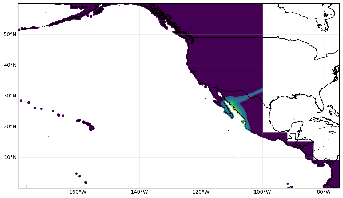
For our analysis, we restrict to the hazard events that affect the land area (defined by the on_land property) in this region:

import shapely
hazard.centroids.region_id = shapely.vectorized.contains(
    region.shape, hazard.centroids.lon, hazard.centroids.lat) & hazard.centroids.on_land.astype(bool)
hazard_EP = hazard.select(reg_id=1)
# Plot one event as an example:
hazard_EP.centroids.plot(c=hazard_EP.intensity[31577,:].toarray().ravel(), s=3);

<cartopy.mpl.geoaxes.GeoAxesSubplot at 0x7f7498568ee0>

Extract events that affect the region of interest

The emulator’s statistics and sampling functionality doesn’t use the Hazard object directly, but an aggregated version of it (a pandas DataFrame). From the Hazard objects, we extract those events that actually “affect” the georegion of interest and store for each the maximum intensity observed within the region (as well as date and location of occurrence):

from climada_petals.hazard.emulator.stats import haz_max_events

# for this example, we regard grid cells as `affected` if they face at least 34 knots wind speeds
KNOTS_2_MS = 0.514444
MIN_WIND_MS = 34 * KNOTS_2_MS

max_events_base = haz_max_events(hazard_EP, min_thresh=MIN_WIND_MS)
max_events_base

2021-03-24 17:46:52,405 - climada.hazard.emulator.stats - INFO - Condensing 45300 hazards to 7401 max events ...

	id	name	year	month	day	lat	lon	intensity
0	1	1	1950	8	17	25.1	-112.3	42.654243
1	5	5	1950	9	3	18.7	-104.0	36.720880
2	8	8	1950	9	17	27.2	-114.0	32.730017
3	13	13	1950	11	24	17.2	-100.6	42.861889
4	17	17	1950	10	26	22.9	-106.3	47.887202
...	...	...	...	...	...	...	...	...
7396	45260	28460	2100	11	21	24.1	-107.0	29.222734
7397	45261	28461	2100	10	25	27.4	-114.2	34.721709
7398	45274	28474	2100	10	20	18.1	-102.1	89.034839
7399	45284	28484	2100	10	9	17.8	-101.5	59.966329
7400	45298	28498	2100	10	13	24.2	-107.5	31.401268

7401 rows × 8 columns

Making draws from the event pool

The most basic functionality of the emulator module is then to subsample from this event pool according to a desired frequency and intensity without taking the date of events into account at all:

from climada_petals.hazard.emulator.emulator import EventPool
event_pool = EventPool(max_events_base)
draws = event_pool.draw_realizations(nrealizations=10, freq_poisson=10, intensity_mean=30, intensity_std=5)

The result draws is a list of nrealizations subsamples from tc_events_pool. The number of events in each sample DataFrame is driven by a Poisson distribution (lambda = 10) and each DataFrame’s mean intensity is 30±5:

assert len(draws) == 10
display(draws[0])
print("Number of events in each sample:", [d.shape[0] for d in draws])
print("Mean intensity of each sample:", [d['intensity'].mean() for d in draws])

	id	name	year	month	day	lat	lon	intensity
754	5285	5285	1967	6	23	18.3	-103.3	30.302091
3458	22096	5296	2023	10	8	15.7	-93.7	47.669055
2357	15416	15416	2001	8	19	22.8	-110.1	30.646163
1329	8892	8892	1979	5	6	19.2	-104.8	39.077807
4153	26512	9712	2038	8	17	31.3	-116.4	18.318382
2131	13949	13949	1996	11	6	18.6	-103.4	34.297652
89	635	635	1952	6	14	21.3	-106.5	51.698398
5106	32250	15450	2057	9	8	21.4	-106.6	37.932184
4703	29808	13008	2049	11	1	59.8	-162.9	20.645396
4844	30510	13710	2051	9	22	26.2	-112.6	26.817070

Number of events in each sample: [10, 7, 11, 7, 10, 13, 11, 16, 12, 6]
Mean intensity of each sample: [33.74041981432531, 32.36753130917463, 34.59815875000344, 31.5348526999235, 33.67298356212818, 27.126272794400833, 34.588544482580225, 32.567385754309875, 33.97376593673842, 33.712914894777875]

Bias-corrected statistics

Now, as noted above, our database actually attaches date information to the events:

import datetime as dt
minyear, maxyear = [dt.datetime.fromordinal(d) for d in [hazard.date.min(), hazard.date.max()]]
print(f"The hazard event database covers the period between {minyear} and {maxyear}.")

The hazard event database covers the period between 1950-01-03 00:00:00 and 2100-12-29 00:00:00.

However, the database contains much more events per year than the underlying physics would suggest. That’s why the creator of the global database provides information about frequency, from which we created the following CSV-data (see last section for more information about the data source and pre-processing steps taken):

import pandas as pd
frequency = pd.read_csv(EMULATOR_DATA_DIR.joinpath("freq_miroc_rcp26.csv"))
with pd.option_context("display.max_rows", 5):
    display(frequency)

	year	freq
0	1950	0.299428
1	1951	0.289091
...	...	...
149	2099	0.348597
150	2100	0.354156

151 rows × 2 columns

The freq column encodes the relative surplus of events for each year: A freq value of 0.29 means that the expected number of events for a particular year is 29, while the actual number of events in the database for that year is 100. Depending on your data provider, it might be more or less simple to derive this kind of information for your event database.

The database might be subject to regional biases: While the whole global event database might represent global statistics of certain physical properties very well, it can still systematically under- or overestimating regionally aggregated properties. One way to “bias-correct” this kind of effect is by comparing with historical records. That’s where a second event database comes in, a database of observed hazard events:

observed = TropCyclone.from_hdf5(EMULATOR_DATA_DIR.joinpath("hazard_360as_ibtracs_1950-2019.hdf5"))
observed.centroids.region_id = shapely.vectorized.contains(
    region.shape, observed.centroids.lon, observed.centroids.lat) & observed.centroids.on_land.astype(bool)
observed_EP = observed.select(reg_id=1)

2021-03-24 17:46:52,543 - climada.hazard.base - INFO - Reading /home/tovogt/.climada/demo/data/emulator/hazard_360as_ibtracs_1950-2019.hdf5

Since the quality of observed data is known to vary a lot in different world regions, we restrict our dataset to an appropriate norm period. Again we condense the hazard object to a DataFrame.

from climada_petals.hazard.emulator.const import TC_BASIN_NORM_PERIOD
norm_period = TC_BASIN_NORM_PERIOD[region.tc_basin[:2]]
observed_EP = observed_EP.select(date=(f"{norm_period[0]}-01-01", f"{norm_period[1]}-12-31"))
max_events_observed = haz_max_events(observed_EP, min_thresh=MIN_WIND_MS)

2021-03-24 17:46:53,013 - climada.hazard.emulator.stats - INFO - Condensing 7335 hazards to 377 max events ...

We would now have all the data for bias correction, but we don’t have to do this manually. The emulator module takes care of this.

Initialize and calibrate the hazard emulator

The most complex part of the emulator module is the HazardEmulator class that automatically applies bias-correction and provides functionality to make draws according to corrected statistics. In the next section, we will see that it can even make draws according to a climate scenario.

from climada_petals.hazard.emulator.emulator import HazardEmulator
em = HazardEmulator(max_events_base, max_events_observed, region, frequency, pool=event_pool)

2021-03-24 17:46:53,188 - climada.hazard.emulator.random - INFO - Results of intensity normalization by subsampling:
2021-03-24 17:46:53,189 - climada.hazard.emulator.random - INFO - - drop 35% of entries satisfying 'intensity > 37.60902402823995'
2021-03-24 17:46:53,189 - climada.hazard.emulator.random - INFO - - mean intensity of simulated events before dropping is 37.6090
2021-03-24 17:46:53,190 - climada.hazard.emulator.random - INFO - - mean intensity of simulated events after dropping is 35.4003
2021-03-24 17:46:53,190 - climada.hazard.emulator.random - INFO - - mean intensity of observed events is 34.6826

All corrections discussed above have already been applied upon initialization and aggregated in the stats attribute (it’s mainly for internal use, so don’t worry if you don’t understand the meaning of all the columns):

em.stats

	year	eventcount	intensity_mean	intensity_std	intensity_max	eventcount_obs	intensity_mean_obs	intensity_std_obs	intensity_max_obs
0	1950	5.041561	37.560036	10.921193	56.148643	3.0	32.444994	4.193251	38.302107
1	1951	4.056249	32.092965	12.225921	61.743472	6.0	21.487378	2.879905	25.614798
2	1952	5.830183	37.488452	15.000097	60.163892	NaN	NaN	NaN	NaN
3	1953	2.185263	33.317693	9.302551	41.871618	3.0	26.853119	2.943347	30.412018
4	1954	3.123722	30.061603	9.982461	37.396814	8.0	29.232035	8.669075	47.533993
...	...	...	...	...	...	...	...	...	...
146	2096	5.641057	39.148745	12.819278	50.586874	NaN	NaN	NaN	NaN
147	2097	7.649071	35.221123	12.889677	55.557459	NaN	NaN	NaN	NaN
148	2098	4.050403	33.088812	12.990415	55.963069	NaN	NaN	NaN	NaN
149	2099	5.217263	34.029102	14.014108	52.617260	NaN	NaN	NaN	NaN
150	2100	7.288148	33.401478	17.953031	68.139491	NaN	NaN	NaN	NaN

151 rows × 9 columns

We can now draw ensembles of events that adhere to the bias-corrected statistics:

# the meaning of `predict_statistics` will be explained in the next section
em.predict_statistics()
draws = em.draw_realizations(10, (2030, 2050))

2021-03-24 17:46:53,222 - climada.hazard.emulator.emulator - INFO - Predicting statistics without climate index predictor...
2021-03-24 17:46:53,226 - climada.hazard.emulator.emulator - INFO - Drawing 10 realizations for period  (2030, 2050)
2030 ... 2050 ... 2050

The returned object draws is a DataFrame with each row corresponding to a storm event from the hazard pool hazard_EP (see above): The column real_id assigns one of 100 realizations to each of the events while the columns id and name are the unique ID and name used in hazard_EP to identify this hazard event. The column year indicates the year in which the event would occur under the hypothetical corrected statistics.

display(draws[:25:2])

	id	name	year	real_id
0	5002	5002	2030	0
2	28485	11685	2030	0
4	8724	8724	2030	2
6	17148	348	2030	2
8	10339	10339	2030	3
10	7026	7026	2030	3
12	27333	10533	2030	5
14	1523	1523	2030	6
16	12183	12183	2030	7
18	20406	3606	2030	8
20	12394	12394	2030	9
22	37101	20301	2031	0
24	17358	558	2031	0

Draw samples according to climate scenario

The emulator can also be used to sample hypothetical events within an arbitrary time period covered by one or several climate index time series:

climate_indices = [pd.read_csv(EMULATOR_DATA_DIR.joinpath("gmt_miroc_rcp26.csv")),
                   pd.read_csv(EMULATOR_DATA_DIR.joinpath("esoi_miroc_rcp26.csv"))]
with pd.option_context("display.max_rows", 5):
    display(*[df for df in climate_indices])

	gmt	year	month
0	0.040892	1861	7
1	0.053463	1862	7
...	...	...	...
437	1.397416	2298	7
438	1.375225	2299	7

439 rows × 3 columns

	esoi	year	month
0	-0.316829	1861	1
1	-0.479121	1861	2
...	...	...	...
5266	-0.569960	2299	11
5267	-0.523571	2299	12

5268 rows × 3 columns

An arbitrary number of climate indices can be provided in a list, each as a DataFrame with a year column and an additional column (in this example, gmt or esoi, respectively) containing the actual climate index data. Optionally, each climate index DataFrame can be at monthly resolution (like in the esoi example), as indicated by an additional month column. A constant month column (like in the gmt example above) will be discarded automatically by the emulator.

Using those climate index time series, we calibrate the emulator, i.e., we determine a statistical connection between climate indices (GMT and ENSO in this example) and tc_events_pool:

em.calibrate_statistics(climate_indices)

Now that the emulator is calibrated, we use GMT and ENSO time series to predict TC statistics under the chosen climate scenario:

em.predict_statistics(climate_indices)

2021-03-24 17:46:54,572 - climada.hazard.emulator.emulator - INFO - Predicting statistics with new climate index time series...

The predicted statistics are stored in the stats_pred attribute of the emulator:

em.stats_pred

	year	gmt	esoi	intensity_mean	intensity_mean_residuals	eventcount	eventcount_residuals
0	1861	0.040892	0.170012	34.803000	2.637305	4.176576	1.272837
1	1862	0.053463	-0.813848	34.038959	2.637305	4.406238	1.272837
2	1863	0.063511	1.040317	35.478856	2.637305	4.018993	1.272837
3	1864	0.061416	1.441388	35.790317	2.637305	3.935384	1.272837
4	1865	0.059797	1.129038	35.547754	2.637305	3.996921	1.272837
...	...	...	...	...	...	...	...
434	2295	1.395940	-0.726180	34.107040	2.637305	6.248324	1.272837
435	2296	1.407416	0.648489	35.174572	2.637305	5.842586	1.272837
436	2297	1.410368	0.769933	35.268883	2.637305	5.811002	1.272837
437	2298	1.397416	0.870595	35.347054	2.637305	5.761524	1.272837
438	2299	1.375225	-0.526354	34.262219	2.637305	6.151251	1.272837

439 rows × 7 columns

Since the climate index time series covers a larger range than our hazard database (1861-2299 vs. 1950-2100), we can even predict the statistics in years that have not been covered by the hazard database.

draws = em.draw_realizations(10, (2110, 2130))
display(draws[:25:2])

2021-03-24 17:46:54,603 - climada.hazard.emulator.emulator - INFO - Drawing 10 realizations for period  (2110, 2130)
2110 ... 2130 ... 2130

	id	name	year	real_id
0	13973	13973	2110	0
2	24253	7453	2110	0
4	14891	14891	2110	0
6	21909	5109	2110	0
8	309	309	2110	1
10	27897	11097	2110	1
12	38751	21951	2110	1
14	31890	15090	2110	1
16	13222	13222	2110	2
18	14662	14662	2110	2
20	9915	9915	2110	2
22	26466	9666	2110	3
24	1523	1523	2110	3

Create sample Hazard object from draws

Using the DataFrame draws, we can produce a hazard object that contains the sampled events from hazard_EP:

hazard_sample = hazard_EP.select(event_names=draws['name'].tolist())

For this event to represent the sample, we need to adjust the date (and, optionally, the frequency according to the number of realizations):

years = [dt.datetime.fromordinal(d).year for d in hazard_sample.date]
hazard_sample.date += [dt.datetime(y_dst, 1, 1).toordinal() - dt.datetime(y, 1, 1).toordinal()
                       for y_dst, y in zip(draws['year'].values, years)]

dates = [dt.datetime.fromordinal(d) for d in hazard_sample.date]
display(dates[:5])
display(dates[-5:])

[datetime.datetime(2110, 7, 26, 0, 0),
 datetime.datetime(2110, 12, 11, 0, 0),
 datetime.datetime(2110, 1, 14, 0, 0),
 datetime.datetime(2110, 7, 26, 0, 0),
 datetime.datetime(2110, 8, 29, 0, 0)]

[datetime.datetime(2130, 7, 29, 0, 0),
 datetime.datetime(2130, 5, 28, 0, 0),
 datetime.datetime(2130, 6, 2, 0, 0),
 datetime.datetime(2130, 9, 13, 0, 0),
 datetime.datetime(2130, 4, 3, 0, 0)]

For the resulting TropCyclone object to be valid, the event names have to be unique. Since our subsampler makes draws for each year and realization independent of any other year and realization, events might occur in more than one year or realization. One way of dealing with this, is the following renaming step:

hazard_EP.event_names = [f"{row.name}-{row.year}-{row.real_id}"
                         for index, row in draws.iterrows()]
hazard_EP.check()

About the input data used for this notebook

Since a crucial ingredient for this module is a (sufficiently large) database of hazard events, executing this tutorial notebook requires external data that is not provided with the official CLIMADA repository. The data is expected to be located in the subdirectory {CONFIG.local_data.demo}/emulator/ according to the CLIMADA config (called EMULATOR_DATA_DIR above). Since parts of the data are under a proprietary license, the data is only available upon request from Thomas Vogt (PIK). In the following, you find a list of all the files used in this notebook with information about sources and pre-processing steps taken:

• ``hazard_360as_miroc_rcp26.hdf5``: A TropCyclone object (stored as 700 MB hdf5-file) that represents the simulated hazard event database. It has been generated from simulated TC tracks provided by Kerry Emanuel for ISIMIP (version 2b). However, since the track data comes with a proprietary license, they are not listed in the official ISIMIP repositories. Tracks for the period 1950-2100 according to the MIROC5 GCM simulations of the RCP 2.6 scenario have been loaded into CLIMADA using the TCTracks.from_simulations_emanuel constructor. The wind fields have been computed from the tracks using CLIMADA’s TropCyclone.from_tracks function and a global set of centroids with 360 arc-seconds (0.1 degree) resolution onland and 1 degree resolution offshore (plotted above).

• ``hazard_360as_ibtracs_1950-2019.hdf5``: A TropCyclone object (stored as 95 MB hdf5-file) that represents the observed hazard event database. It has been generated from records in the IBTrACS database for the years 1950-2019. The tracks have been loaded into CLIMADA using the TCTracks.from_ibtracs_netcdf constructor. Then, wind fields have been computed as for the simulated tracks (see hazard_360as_miroc_rcp26.hdf5).

• ``freq_miroc_rcp26.csv``: A table with year and freq column covering the years 1950-2100. The freq values have been obtained by dividing the freqyear field contained in the simulated TC tracks (see hazard_360as_miroc_rcp26.hdf5) by 300 (the total number of global tracks per year in the simulated TC track files).

• ``gmt_miroc_rcp26.csv``: A table with gmt, year and month field (the month is constantly set to 7). GMT stands for “Global Mean (surface) Temperature”. The CMIP5 monthly mean atmopsheric (Amon) tas temperature field of MIROC5 RCP 2.6 simulations covering the years 1861-2299 has been averaged globally and annually using the data processing tool CDO. The data is relative to the mean over the 500 year pre-industrial control run of the GCM and the time series has been smoothed by applying a 21-year running mean.

• ``esoi_miroc_rcp26.csv``: A table with esoi, year and month field. ESOI stands for “Equatorial Southern Oscillation Index”. Instructions on how to compute this index from air pressure can be found on the ENSO Monitoring website, hosted by Columbia University. For the air pressure input, we extracted the CMIP5 monthly mean atmopsheric (Amon) psl field of MIROC5 RCP 2.6 simulations covering the years 1861-2299.