River Flood based on GloFAS Discharge Data

This tutorial will guide through the process of computing flood foodprints from GloFAS river discharge data and using these footprints in CLIMADA impact calculations.

Executing this tutorial requires access to the Copernicus Data Store (CDS) and the input data for the flood footprint pipeline. Please have a look at the documentation of the GloFAS River Flood module and follow the instructions in its “Preparation” section before continuing.

The first step is setting up the “static” data required for the river flood model. The setup_all() function will download the flood hazard maps, the FLOPROS flood protection database, and the pre-computed Gumbel distribution fit parameters. This might take a while.

from climada.util import log_level
from climada_petals.hazard.rf_glofas import setup_all

with log_level("DEBUG", "climada_petals"):
    setup_all()

/home/roo/miniforge3/envs/climada_flood/lib/python3.9/site-packages/dask/dataframe/_pyarrow_compat.py:17: FutureWarning: Minimal version of pyarrow will soon be increased to 14.0.1. You are using 12.0.1. Please consider upgrading.
  warnings.warn(

2024-02-29 14:54:26,872 - climada_petals.hazard.rf_glofas.setup - DEBUG - Rewriting flood hazard maps to NetCDF files
2024-02-29 14:54:26,873 - climada_petals.hazard.rf_glofas.setup - DEBUG - Merging flood hazard maps into single dataset
2024-02-29 14:58:21,780 - climada_petals.hazard.rf_glofas.setup - DEBUG - Downloading FLOPROS database
2024-02-29 14:58:22,371 - climada_petals.hazard.rf_glofas.setup - DEBUG - Downloading Gumbel fit parameters

from climada_petals.hazard.rf_glofas import RiverFloodInundation

countries = ["Germany", "Switzerland", "Austria"]

rf = RiverFloodInundation()
rf.download_forecast(
    countries=countries,
    forecast_date="2021-07-10",
    preprocess=lambda x: x.max(dim="step"),
    system_version="operational",  # Version mislabeled
)

ds_flood = rf.compute()
ds_flood

/home/roo/miniforge3/envs/climada_flood/lib/python3.9/site-packages/xarray/core/dataset.py:282: UserWarning: The specified chunks separate the stored chunks along dimension "latitude" starting at index 1377. This could degrade performance. Instead, consider rechunking after loading.
  warnings.warn(
/home/roo/miniforge3/envs/climada_flood/lib/python3.9/site-packages/xarray/core/dataset.py:282: UserWarning: The specified chunks separate the stored chunks along dimension "longitude" starting at index 3480. This could degrade performance. Instead, consider rechunking after loading.
  warnings.warn(

2024-02-29 14:58:26,019 - climada_petals.hazard.rf_glofas.cds_glofas_downloader - INFO - Skipping request for file '/home/roo/climada/data/cds-download/240229-145826-83e84eba8992a4a4d5f8af0a923e2458.grib' because it already exists

/home/roo/miniforge3/envs/climada_flood/lib/python3.9/site-packages/dask/array/routines.py:325: PerformanceWarning: Increasing number of chunks by factor of 50
  intermediate = blockwise(

<xarray.Dataset>
Dimensions:              (number: 50, time: 1, longitude: 1356, latitude: 1128)
Coordinates:
  * number               (number) int64 1 2 3 4 5 6 7 8 ... 44 45 46 47 48 49 50
  * time                 (time) datetime64[ns] 2021-07-10
    surface              float64 ...
    step                 timedelta64[ns] ...
  * longitude            (longitude) float64 5.854 5.863 5.871 ... 17.14 17.15
  * latitude             (latitude) float64 55.15 55.14 55.13 ... 45.76 45.75
Data variables:
    flood_depth          (latitude, longitude, time, number) float32 dask.array<chunksize=(762, 162, 1, 50), meta=np.ndarray>
    flood_depth_flopros  (latitude, longitude, time, number) float32 dask.array<chunksize=(762, 162, 1, 50), meta=np.ndarray>

xarray.Dataset

• Dimensions:
  • number: 50
  • time: 1
  • longitude: 1356
  • latitude: 1128
• Coordinates: (6)
  • number
    (number)
    int64
    1 2 3 4 5 6 7 ... 45 46 47 48 49 50

    array([ 1,  2,  3,  4,  5,  6,  7,  8,  9, 10, 11, 12, 13, 14, 15, 16, 17, 18,
           19, 20, 21, 22, 23, 24, 25, 26, 27, 28, 29, 30, 31, 32, 33, 34, 35, 36,
           37, 38, 39, 40, 41, 42, 43, 44, 45, 46, 47, 48, 49, 50])

  • time
    (time)
    datetime64[ns]
    2021-07-10

    array(['2021-07-10T00:00:00.000000000'], dtype='datetime64[ns]')

  • surface
    ()
    float64
    ...

    [1 values with dtype=float64]

  • step
    ()
    timedelta64[ns]
    ...

    [1 values with dtype=timedelta64[ns]]

  • longitude
    (longitude)
    float64
    5.854 5.863 5.871 ... 17.14 17.15

    array([ 5.854179,  5.862512,  5.870846, ..., 17.129179, 17.137512, 17.145846])

  • latitude
    (latitude)
    float64
    55.15 55.14 55.13 ... 45.76 45.75

    array([55.145931, 55.137598, 55.129264, ..., 45.770931, 45.762598, 45.754264])

• Data variables: (2)
  • flood_depth
    (latitude, longitude, time, number)
    float32
    dask.array<chunksize=(762, 162, 1, 50), meta=np.ndarray>

    Array Chunk Bytes 291.74 MiB 128.04 MiB Shape (1128, 1356, 1, 50) (762, 881, 1, 50) Dask graph 9 chunks in 14 graph layers Data type float32 numpy.ndarray

  • flood_depth_flopros
    (latitude, longitude, time, number)
    float32
    dask.array<chunksize=(762, 162, 1, 50), meta=np.ndarray>

    Array Chunk Bytes 291.74 MiB 128.04 MiB Shape (1128, 1356, 1, 50) (762, 881, 1, 50) Dask graph 9 chunks in 14 graph layers Data type float32 numpy.ndarray

• Indexes: (4)
  • number
    PandasIndex

    PandasIndex(Index([ 1,  2,  3,  4,  5,  6,  7,  8,  9, 10, 11, 12, 13, 14, 15, 16, 17, 18,
           19, 20, 21, 22, 23, 24, 25, 26, 27, 28, 29, 30, 31, 32, 33, 34, 35, 36,
           37, 38, 39, 40, 41, 42, 43, 44, 45, 46, 47, 48, 49, 50],
          dtype='int64', name='number'))

  • time
    PandasIndex

    PandasIndex(DatetimeIndex(['2021-07-10'], dtype='datetime64[ns]', name='time', freq=None))

  • longitude
    PandasIndex

    PandasIndex(Index([ 5.854178873691012,  5.862512207024338,  5.870845540357664,
            5.879178873691018, 5.8875122070243435,  5.895845540357669,
            5.904178873690995,  5.912512207024349,  5.920845540357675,
            5.929178873691001,
           ...
           17.070845540357226,  17.07917887369055, 17.087512207023906,
            17.09584554035723, 17.104178873690557, 17.112512207023883,
           17.120845540357237, 17.129178873690563,  17.13751220702389,
           17.145845540357215],
          dtype='float64', name='longitude', length=1356))

  • latitude
    PandasIndex

    PandasIndex(Index([ 55.14593098958446,  55.13759765625113,  55.12926432291779,
           55.120930989584465, 55.112597656251125,   55.1042643229178,
            55.09593098958446,  55.08759765625113, 55.079264322917794,
            55.07093098958446,
           ...
            45.82926432291816,  45.82093098958483,   45.8125976562515,
           45.804264322918165,  45.79593098958483,   45.7875976562515,
           45.779264322918166,  45.77093098958483,   45.7625976562515,
            45.75426432291817],
          dtype='float64', name='latitude', length=1128))

• Attributes: (0)

The returned dataset contains two variables, flood_depth and flood_depth_flopros which indicate the flood footprints without and with FLOPROS protection levels considered, respectively. Notice that intermediate data is stored in a cache directory by default, but the returned flood data is not. You can use save_file() to store it. The cache directory will be deleted as soon as the RiverFloodInundation object is.

from climada_petals.hazard.rf_glofas import save_file

save_file(ds_flood, "flood-2021-07-10.nc")

To use the data within CLIMADA we will have to “translate” it into a Hazard object. We provide a helper function for that: climada_petals.hazard.rf_glofas.rf_glofas.hazard_series_from_dataset(). Here we have to specify the variable to be read as hazard intensity (we choose the one without FLOPROS protection levels) and the dimension of the dataset that indicates the “event” dimension of the Hazard object. If the dataset contained more dimensions than event_dim, latitude and longitude, the function hazard_series_from_dataset would return a pandas Series of Hazard objects indexed with these additional dimensions. We will see this later.

Notice that storing data and reading it from a file might in some cases be faster than loading the data directly into a Hazard object, because the latter requires some potentially costly transpositions of the underlying data structures.

from climada_petals.hazard.rf_glofas import hazard_series_from_dataset

hazard = hazard_series_from_dataset(
    ds_flood, intensity="flood_depth", event_dim="number"
)[0]
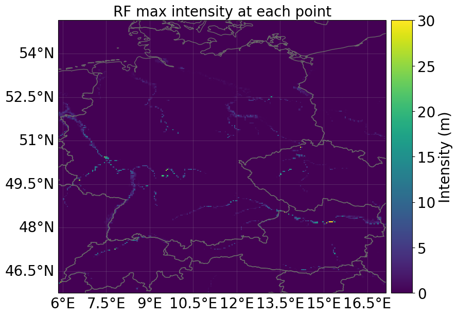
hazard.plot_intensity(event=0)

2024-02-29 14:59:26,406 - climada.hazard.base - WARNING - Failed to read values of 'number' as dates. Hazard.event_name will be empty strings

/tmp/ipykernel_41108/360336388.py:3: FutureWarning: Series.__getitem__ treating keys as positions is deprecated. In a future version, integer keys will always be treated as labels (consistent with DataFrame behavior). To access a value by position, use `ser.iloc[pos]`
  hazard = hazard_series_from_dataset(

<GeoAxes: title={'center': 'RF max intensity at each point'}>

Exposure and Vulnerability

When looking at flood warnings and protection we typically want to determine how many people might be affected from floods or lose their homes. We therefore use data on population distribution as exposure. To that end, we create a LitPop exposure with the pop mode for the countries of interest.

Being affected by a flood can be considered a binary classification (yes/no), therefore we use a simple step function with a relatively low threshold of 0.2 m.

Notice that we set the impact function identifier to "RF" because this is the hazard type identifier of RiverFlood.

from climada.entity import LitPop
from climada.entity import ImpactFunc, ImpactFuncSet

# Create a population exposure
exposure = LitPop.from_population(["Germany", "Switzerland", "Austria"])
exposure.gdf["impf_RF"] = 1

# Create a impact function for being affected by flooding
impf_affected = ImpactFunc.from_step_impf(
    intensity=(0.0, 0.2, 100.0), impf_id=1, haz_type="RF"
)
impf_set_affected = ImpactFuncSet([impf_affected])

2024-02-29 14:59:53,885 - climada.entity.exposures.litpop.litpop - INFO - 
 LitPop: Init Exposure for country: DEU (276)...

2024-02-29 14:59:53,935 - climada.entity.exposures.litpop.gpw_population - WARNING - Reference year: 2018. Using nearest available year for GPW data: 2020
2024-02-29 14:59:53,936 - climada.entity.exposures.litpop.gpw_population - INFO - GPW Version v4.11
2024-02-29 14:59:53,956 - climada.entity.exposures.litpop.gpw_population - WARNING - Reference year: 2018. Using nearest available year for GPW data: 2020
2024-02-29 14:59:53,957 - climada.entity.exposures.litpop.gpw_population - INFO - GPW Version v4.11
2024-02-29 14:59:53,982 - climada.entity.exposures.litpop.gpw_population - WARNING - Reference year: 2018. Using nearest available year for GPW data: 2020
2024-02-29 14:59:53,983 - climada.entity.exposures.litpop.gpw_population - INFO - GPW Version v4.11
2024-02-29 14:59:54,006 - climada.entity.exposures.litpop.gpw_population - WARNING - Reference year: 2018. Using nearest available year for GPW data: 2020
2024-02-29 14:59:54,007 - climada.entity.exposures.litpop.gpw_population - INFO - GPW Version v4.11
2024-02-29 14:59:54,031 - climada.entity.exposures.litpop.gpw_population - WARNING - Reference year: 2018. Using nearest available year for GPW data: 2020
2024-02-29 14:59:54,032 - climada.entity.exposures.litpop.gpw_population - INFO - GPW Version v4.11
2024-02-29 14:59:54,058 - climada.entity.exposures.litpop.gpw_population - WARNING - Reference year: 2018. Using nearest available year for GPW data: 2020
2024-02-29 14:59:54,059 - climada.entity.exposures.litpop.gpw_population - INFO - GPW Version v4.11
2024-02-29 14:59:54,084 - climada.entity.exposures.litpop.gpw_population - WARNING - Reference year: 2018. Using nearest available year for GPW data: 2020
2024-02-29 14:59:54,085 - climada.entity.exposures.litpop.gpw_population - INFO - GPW Version v4.11
2024-02-29 14:59:54,104 - climada.entity.exposures.litpop.gpw_population - WARNING - Reference year: 2018. Using nearest available year for GPW data: 2020
2024-02-29 14:59:54,105 - climada.entity.exposures.litpop.gpw_population - INFO - GPW Version v4.11
2024-02-29 14:59:54,134 - climada.entity.exposures.litpop.gpw_population - WARNING - Reference year: 2018. Using nearest available year for GPW data: 2020
2024-02-29 14:59:54,135 - climada.entity.exposures.litpop.gpw_population - INFO - GPW Version v4.11
2024-02-29 14:59:54,151 - climada.entity.exposures.litpop.gpw_population - WARNING - Reference year: 2018. Using nearest available year for GPW data: 2020
2024-02-29 14:59:54,151 - climada.entity.exposures.litpop.gpw_population - INFO - GPW Version v4.11
2024-02-29 14:59:54,185 - climada.entity.exposures.litpop.gpw_population - WARNING - Reference year: 2018. Using nearest available year for GPW data: 2020
2024-02-29 14:59:54,186 - climada.entity.exposures.litpop.gpw_population - INFO - GPW Version v4.11
2024-02-29 14:59:56,052 - climada.entity.exposures.litpop.gpw_population - WARNING - Reference year: 2018. Using nearest available year for GPW data: 2020
2024-02-29 14:59:56,053 - climada.entity.exposures.litpop.gpw_population - INFO - GPW Version v4.11
2024-02-29 14:59:56,119 - climada.entity.exposures.litpop.gpw_population - WARNING - Reference year: 2018. Using nearest available year for GPW data: 2020
2024-02-29 14:59:56,120 - climada.entity.exposures.litpop.gpw_population - INFO - GPW Version v4.11
2024-02-29 14:59:56,194 - climada.entity.exposures.litpop.gpw_population - WARNING - Reference year: 2018. Using nearest available year for GPW data: 2020
2024-02-29 14:59:56,195 - climada.entity.exposures.litpop.gpw_population - INFO - GPW Version v4.11
2024-02-29 14:59:56,257 - climada.entity.exposures.litpop.gpw_population - WARNING - Reference year: 2018. Using nearest available year for GPW data: 2020
2024-02-29 14:59:56,258 - climada.entity.exposures.litpop.gpw_population - INFO - GPW Version v4.11
2024-02-29 14:59:56,339 - climada.entity.exposures.litpop.gpw_population - WARNING - Reference year: 2018. Using nearest available year for GPW data: 2020
2024-02-29 14:59:56,340 - climada.entity.exposures.litpop.gpw_population - INFO - GPW Version v4.11
2024-02-29 14:59:56,411 - climada.entity.exposures.litpop.gpw_population - WARNING - Reference year: 2018. Using nearest available year for GPW data: 2020
2024-02-29 14:59:56,412 - climada.entity.exposures.litpop.gpw_population - INFO - GPW Version v4.11
2024-02-29 14:59:56,478 - climada.entity.exposures.litpop.gpw_population - WARNING - Reference year: 2018. Using nearest available year for GPW data: 2020
2024-02-29 14:59:56,479 - climada.entity.exposures.litpop.gpw_population - INFO - GPW Version v4.11
2024-02-29 14:59:56,541 - climada.entity.exposures.litpop.gpw_population - WARNING - Reference year: 2018. Using nearest available year for GPW data: 2020
2024-02-29 14:59:56,542 - climada.entity.exposures.litpop.gpw_population - INFO - GPW Version v4.11
2024-02-29 14:59:56,614 - climada.entity.exposures.litpop.gpw_population - WARNING - Reference year: 2018. Using nearest available year for GPW data: 2020
2024-02-29 14:59:56,615 - climada.entity.exposures.litpop.gpw_population - INFO - GPW Version v4.11
2024-02-29 14:59:56,685 - climada.entity.exposures.litpop.gpw_population - WARNING - Reference year: 2018. Using nearest available year for GPW data: 2020
2024-02-29 14:59:56,687 - climada.entity.exposures.litpop.gpw_population - INFO - GPW Version v4.11
2024-02-29 14:59:58,417 - climada.entity.exposures.litpop.litpop - INFO - 
 LitPop: Init Exposure for country: CHE (756)...

2024-02-29 15:00:00,409 - climada.entity.exposures.litpop.litpop - INFO - 
 LitPop: Init Exposure for country: AUT (40)...

2024-02-29 15:00:01,222 - climada.entity.exposures.base - INFO - Hazard type not set in impf_
2024-02-29 15:00:01,223 - climada.entity.exposures.base - INFO - category_id not set.
2024-02-29 15:00:01,224 - climada.entity.exposures.base - INFO - cover not set.
2024-02-29 15:00:01,224 - climada.entity.exposures.base - INFO - deductible not set.
2024-02-29 15:00:01,225 - climada.entity.exposures.base - INFO - centr_ not set.

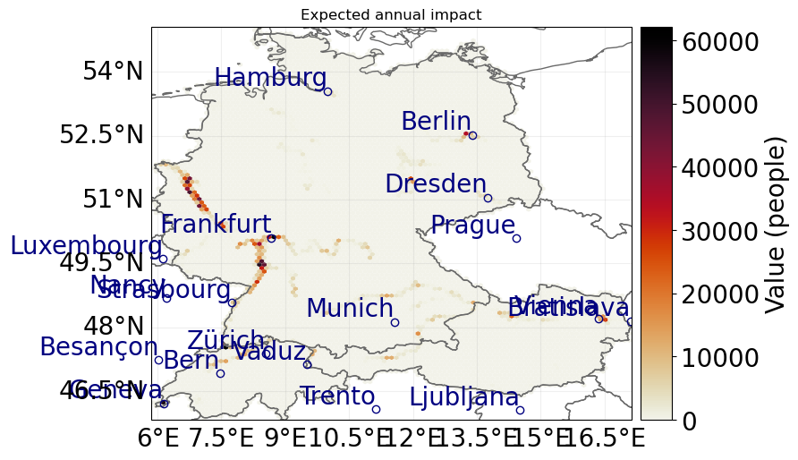
Impact Calculation

We simply plug everything together and calculate the impact. Afterwards, we plot the average impact for 14 July 2021.

The averaging function takes the frequency parameter of the hazard into account. By default, all hazard events have a frequency of 1. This may result in unexpected values for average impacts. We therefore divide the frequency by the number of events before plotting.

import numpy as np
from climada.engine import ImpactCalc

hazard.frequency = hazard.frequency / hazard.size
impact = ImpactCalc(exposure, impf_set_affected, hazard).impact()
impact.plot_hexbin_eai_exposure(gridsize=100, lw=0)

2024-02-29 15:00:01,268 - climada.entity.exposures.base - INFO - Matching 876313 exposures with 1529568 centroids.
2024-02-29 15:00:01,281 - climada.util.coordinates - INFO - No exact centroid match found. Reprojecting coordinates to nearest neighbor closer than the threshold = 100
2024-02-29 15:00:03,547 - climada.engine.impact_calc - INFO - Calculating impact for 2606616 assets (>0) and 50 events.

<GeoAxes: title={'center': 'Expected annual impact'}>

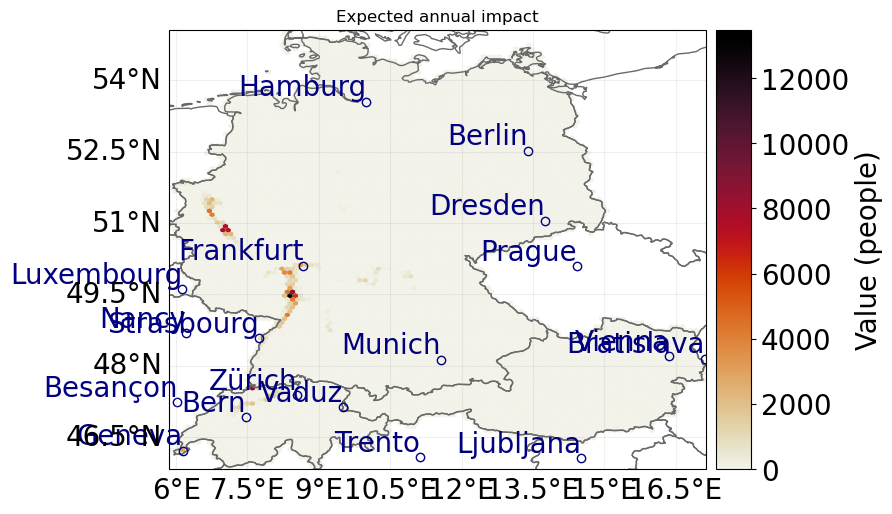
FLOPROS Database Protection Standards

So far, we ignored any protection standards, likely overestimating the impact of events. The FLOPROS database provides information on river flood protection standards. It is a supplement to the publication by P. Scussolini et al.: “FLOPROS: an evolving global database of flood protection standards” It was automatically loaded when you called setup_all().

Let’s compare the hazard and corresponding impacts when considering the FLOPROS protection standards!

hazard_flopros = hazard_series_from_dataset(
    ds_flood, intensity="flood_depth_flopros", event_dim="number"
)[0]
hazard_flopros.plot_intensity(event=0)

2024-02-29 15:00:09,411 - climada.hazard.base - WARNING - Failed to read values of 'number' as dates. Hazard.event_name will be empty strings

/tmp/ipykernel_41108/1832447213.py:1: FutureWarning: Series.__getitem__ treating keys as positions is deprecated. In a future version, integer keys will always be treated as labels (consistent with DataFrame behavior). To access a value by position, use `ser.iloc[pos]`
  hazard_flopros = hazard_series_from_dataset(

<GeoAxes: title={'center': 'RF max intensity at each point'}>

hazard_flopros.frequency = hazard_flopros.frequency / hazard_flopros.size
impact_flopros = ImpactCalc(exposure, impf_set_affected, hazard_flopros).impact()
impact_flopros.plot_hexbin_eai_exposure(gridsize=100, lw=0)

2024-02-29 15:00:37,496 - climada.entity.exposures.base - INFO - Exposures matching centroids already found for RF
2024-02-29 15:00:37,497 - climada.entity.exposures.base - INFO - Existing centroids will be overwritten for RF
2024-02-29 15:00:37,498 - climada.entity.exposures.base - INFO - Matching 876313 exposures with 1529568 centroids.
2024-02-29 15:00:37,514 - climada.util.coordinates - INFO - No exact centroid match found. Reprojecting coordinates to nearest neighbor closer than the threshold = 100
2024-02-29 15:00:39,504 - climada.engine.impact_calc - INFO - Calculating impact for 2606616 assets (>0) and 50 events.

<GeoAxes: title={'center': 'Expected annual impact'}>

import pandas as pd
import matplotlib.pyplot as plt

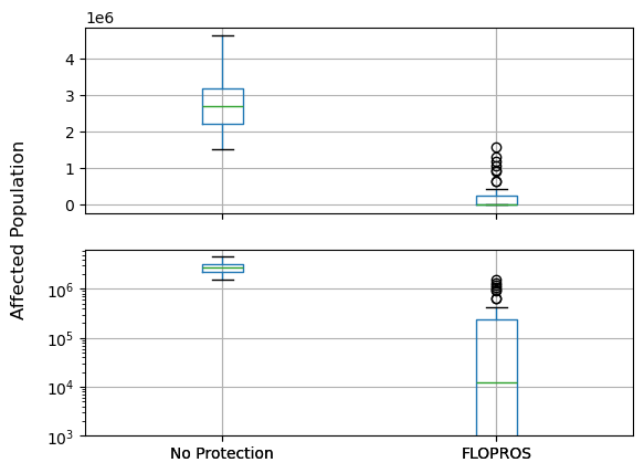
df_impact = pd.DataFrame.from_dict(
    data={"No Protection": impact.at_event, "FLOPROS": impact_flopros.at_event}
)

fig, axes = plt.subplots(2, 1, sharex=True)

for ax in axes:
    df_impact.boxplot(ax=ax)

axes[1].set_yscale("log")
axes[1].set_ylim(bottom=1e3)
fig.supylabel("Affected Population")

Text(0.02, 0.5, 'Affected Population')

Multidimensional Data

We computed the risk of population being affected by 0.2 m of river flooding from the forecast issued on 2021-07-10 over the next 10 days. We reduced the dimensionality of the data by simply taking the maximum discharge over the lead time of 10 days before computing the flood footprint. We can get a clearer picture of flood timings by defining sub-selection of the lead time and computing footprints for each of these. This is easy to do because we receive the downloaded discharge as xarray DataArray and can manipulate it however we like before putting it into the computation pipeline. However, increasing the amount of flood footprints to compute will also increase the computational cost.

discharge = rf.download_forecast(
    countries=countries,
    forecast_date="2021-07-10",
    system_version="operational",  # Version mislabeled
)
discharge

2024-02-29 15:00:44,793 - climada_petals.hazard.rf_glofas.cds_glofas_downloader - INFO - Skipping request for file '/home/roo/climada/data/cds-download/240229-150044-83e84eba8992a4a4d5f8af0a923e2458.grib' because it already exists

<xarray.DataArray 'dis24' (time: 1, number: 50, step: 10, latitude: 95,
                           longitude: 114)>
dask.array<broadcast_to, shape=(1, 50, 10, 95, 114), dtype=float32, chunksize=(1, 50, 10, 95, 114), chunktype=numpy.ndarray>
Coordinates:
  * number      (number) int64 1 2 3 4 5 6 7 8 9 ... 42 43 44 45 46 47 48 49 50
  * time        (time) datetime64[ns] 2021-07-10
  * step        (step) timedelta64[ns] 1 days 2 days 3 days ... 9 days 10 days
    surface     float64 ...
  * latitude    (latitude) float64 55.15 55.05 54.95 54.85 ... 45.95 45.85 45.75
  * longitude   (longitude) float64 5.85 5.95 6.05 6.15 ... 16.95 17.05 17.15
    valid_time  (step) datetime64[ns] dask.array<chunksize=(10,), meta=np.ndarray>
Attributes: (12/30)
    GRIB_paramId:                             240024
    GRIB_dataType:                            pf
    GRIB_numberOfPoints:                      10830
    GRIB_typeOfLevel:                         surface
    GRIB_stepUnits:                           1
    GRIB_stepType:                            avg
    ...                                       ...
    GRIB_shortName:                           dis24
    GRIB_totalNumber:                         51
    GRIB_units:                               m**3 s**-1
    long_name:                                Mean discharge in the last 24 h...
    units:                                    m**3 s**-1
    standard_name:                            unknown

xarray.DataArray

'dis24'

• time: 1
• number: 50
• step: 10
• latitude: 95
• longitude: 114

• dask.array<chunksize=(1, 50, 10, 95, 114), meta=np.ndarray>

  Array Chunk Bytes 20.66 MiB 20.66 MiB Shape (1, 50, 10, 95, 114) (1, 50, 10, 95, 114) Dask graph 1 chunks in 3 graph layers Data type float32 numpy.ndarray

• Coordinates: (7)
  • number
    (number)
    int64
    1 2 3 4 5 6 7 ... 45 46 47 48 49 50

    long_name :

    ensemble member numerical id

    units :

    1

    standard_name :

    realization

    array([ 1,  2,  3,  4,  5,  6,  7,  8,  9, 10, 11, 12, 13, 14, 15, 16, 17, 18,
           19, 20, 21, 22, 23, 24, 25, 26, 27, 28, 29, 30, 31, 32, 33, 34, 35, 36,
           37, 38, 39, 40, 41, 42, 43, 44, 45, 46, 47, 48, 49, 50])

  • time
    (time)
    datetime64[ns]
    2021-07-10

    long_name :

    initial time of forecast

    standard_name :

    forecast_reference_time

    array(['2021-07-10T00:00:00.000000000'], dtype='datetime64[ns]')

  • step
    (step)
    timedelta64[ns]
    1 days 2 days ... 9 days 10 days

    long_name :

    time since forecast_reference_time

    standard_name :

    forecast_period

    array([ 86400000000000, 172800000000000, 259200000000000, 345600000000000,
           432000000000000, 518400000000000, 604800000000000, 691200000000000,
           777600000000000, 864000000000000], dtype='timedelta64[ns]')

  • surface
    ()
    float64
    ...

    long_name :

    original GRIB coordinate for key: level(surface)

    units :

    1

    [1 values with dtype=float64]

  • latitude
    (latitude)
    float64
    55.15 55.05 54.95 ... 45.85 45.75

    units :

    degrees_north

    standard_name :

    latitude

    long_name :

    latitude

    stored_direction :

    decreasing

    array([55.15, 55.05, 54.95, 54.85, 54.75, 54.65, 54.55, 54.45, 54.35, 54.25,
           54.15, 54.05, 53.95, 53.85, 53.75, 53.65, 53.55, 53.45, 53.35, 53.25,
           53.15, 53.05, 52.95, 52.85, 52.75, 52.65, 52.55, 52.45, 52.35, 52.25,
           52.15, 52.05, 51.95, 51.85, 51.75, 51.65, 51.55, 51.45, 51.35, 51.25,
           51.15, 51.05, 50.95, 50.85, 50.75, 50.65, 50.55, 50.45, 50.35, 50.25,
           50.15, 50.05, 49.95, 49.85, 49.75, 49.65, 49.55, 49.45, 49.35, 49.25,
           49.15, 49.05, 48.95, 48.85, 48.75, 48.65, 48.55, 48.45, 48.35, 48.25,
           48.15, 48.05, 47.95, 47.85, 47.75, 47.65, 47.55, 47.45, 47.35, 47.25,
           47.15, 47.05, 46.95, 46.85, 46.75, 46.65, 46.55, 46.45, 46.35, 46.25,
           46.15, 46.05, 45.95, 45.85, 45.75])

  • longitude
    (longitude)
    float64
    5.85 5.95 6.05 ... 17.05 17.15

    units :

    degrees_east

    standard_name :

    longitude

    long_name :

    longitude

    array([ 5.85,  5.95,  6.05,  6.15,  6.25,  6.35,  6.45,  6.55,  6.65,  6.75,
            6.85,  6.95,  7.05,  7.15,  7.25,  7.35,  7.45,  7.55,  7.65,  7.75,
            7.85,  7.95,  8.05,  8.15,  8.25,  8.35,  8.45,  8.55,  8.65,  8.75,
            8.85,  8.95,  9.05,  9.15,  9.25,  9.35,  9.45,  9.55,  9.65,  9.75,
            9.85,  9.95, 10.05, 10.15, 10.25, 10.35, 10.45, 10.55, 10.65, 10.75,
           10.85, 10.95, 11.05, 11.15, 11.25, 11.35, 11.45, 11.55, 11.65, 11.75,
           11.85, 11.95, 12.05, 12.15, 12.25, 12.35, 12.45, 12.55, 12.65, 12.75,
           12.85, 12.95, 13.05, 13.15, 13.25, 13.35, 13.45, 13.55, 13.65, 13.75,
           13.85, 13.95, 14.05, 14.15, 14.25, 14.35, 14.45, 14.55, 14.65, 14.75,
           14.85, 14.95, 15.05, 15.15, 15.25, 15.35, 15.45, 15.55, 15.65, 15.75,
           15.85, 15.95, 16.05, 16.15, 16.25, 16.35, 16.45, 16.55, 16.65, 16.75,
           16.85, 16.95, 17.05, 17.15])

  • valid_time
    (step)
    datetime64[ns]
    dask.array<chunksize=(10,), meta=np.ndarray>

    standard_name :

    time

    long_name :

    time

    Array Chunk Bytes 80 B 80 B Shape (10,) (10,) Dask graph 1 chunks in 2 graph layers Data type datetime64[ns] numpy.ndarray

• Indexes: (5)
  • number
    PandasIndex

    PandasIndex(Index([ 1,  2,  3,  4,  5,  6,  7,  8,  9, 10, 11, 12, 13, 14, 15, 16, 17, 18,
           19, 20, 21, 22, 23, 24, 25, 26, 27, 28, 29, 30, 31, 32, 33, 34, 35, 36,
           37, 38, 39, 40, 41, 42, 43, 44, 45, 46, 47, 48, 49, 50],
          dtype='int64', name='number'))

  • time
    PandasIndex

    PandasIndex(DatetimeIndex(['2021-07-10'], dtype='datetime64[ns]', name='time', freq=None))

  • step
    PandasIndex

    PandasIndex(TimedeltaIndex([ '1 days',  '2 days',  '3 days',  '4 days',  '5 days',
                     '6 days',  '7 days',  '8 days',  '9 days', '10 days'],
                   dtype='timedelta64[ns]', name='step', freq=None))

  • latitude
    PandasIndex

    PandasIndex(Index([             55.15,              55.05, 54.949999999999996,
           54.849999999999994,  54.74999999999999,  54.64999999999999,
            54.54999999999999,  54.44999999999999,  54.34999999999999,
           54.249999999999986, 54.149999999999984,  54.04999999999998,
            53.94999999999998,  53.84999999999998,  53.74999999999998,
            53.64999999999998, 53.549999999999976, 53.449999999999974,
            53.34999999999997,  53.24999999999997,  53.14999999999997,
            53.04999999999997,  52.94999999999997, 52.849999999999966,
           52.749999999999964,  52.64999999999996,  52.54999999999996,
            52.44999999999996,  52.34999999999996,  52.24999999999996,
           52.149999999999956, 52.049999999999955,  51.94999999999995,
            51.84999999999995,  51.74999999999995,  51.64999999999995,
            51.54999999999995, 51.449999999999946, 51.349999999999945,
            51.24999999999994,  51.14999999999994,  51.04999999999994,
            50.94999999999994,  50.84999999999994, 50.749999999999936,
           50.649999999999935,  50.54999999999993,  50.44999999999993,
            50.34999999999993,  50.24999999999993,  50.14999999999993,
           50.049999999999926, 49.949999999999925,  49.84999999999992,
            49.74999999999992,  49.64999999999992,  49.54999999999992,
            49.44999999999992, 49.349999999999916, 49.249999999999915,
            49.14999999999991,  49.04999999999991,  48.94999999999991,
            48.84999999999991,  48.74999999999991, 48.649999999999906,
           48.549999999999905,   48.4499999999999,   48.3499999999999,
             48.2499999999999,   48.1499999999999,   48.0499999999999,
           47.949999999999896, 47.849999999999895,  47.74999999999989,
            47.64999999999989,  47.54999999999989,  47.44999999999989,
            47.34999999999989, 47.249999999999886, 47.149999999999885,
            47.04999999999988,  46.94999999999988,  46.84999999999988,
            46.74999999999988,  46.64999999999988, 46.549999999999876,
           46.449999999999875,  46.34999999999987,  46.24999999999987,
            46.14999999999987,  46.04999999999987,  45.94999999999987,
           45.849999999999866,              45.75],
          dtype='float64', name='latitude'))

  • longitude
    PandasIndex

    PandasIndex(Index([              5.85,  5.949999999999999,  6.049999999999999,
            6.149999999999999,  6.249999999999998,  6.349999999999998,
           6.4499999999999975,  6.549999999999997,  6.649999999999997,
           6.7499999999999964,
           ...
           16.249999999999968,  16.34999999999997,  16.44999999999997,
           16.549999999999972, 16.649999999999974, 16.749999999999975,
           16.849999999999977, 16.949999999999978,  17.04999999999998,
                        17.15],
          dtype='float64', name='longitude', length=114))

• Attributes: (30)

  GRIB_paramId :

  240024

  GRIB_dataType :

  pf

  GRIB_numberOfPoints :

  10830

  GRIB_typeOfLevel :

  surface

  GRIB_stepUnits :

  1

  GRIB_stepType :

  avg

  GRIB_gridType :

  regular_ll

  GRIB_NV :

  0

  GRIB_Nx :

  114

  GRIB_Ny :

  95

  GRIB_cfName :

  unknown

  GRIB_cfVarName :

  dis24

  GRIB_gridDefinitionDescription :

  Latitude/longitude

  GRIB_iDirectionIncrementInDegrees :

  0.1

  GRIB_iScansNegatively :

  0

  GRIB_jDirectionIncrementInDegrees :

  0.1

  GRIB_jPointsAreConsecutive :

  0

  GRIB_jScansPositively :

  0

  GRIB_latitudeOfFirstGridPointInDegrees :

  55.15

  GRIB_latitudeOfLastGridPointInDegrees :

  45.75

  GRIB_longitudeOfFirstGridPointInDegrees :

  5.85

  GRIB_longitudeOfLastGridPointInDegrees :

  17.15

  GRIB_missingValue :

  9999

  GRIB_name :

  Mean discharge in the last 24 hours

  GRIB_shortName :

  dis24

  GRIB_totalNumber :

  51

  GRIB_units :

  m**3 s**-1

  long_name :

  Mean discharge in the last 24 hours

  units :

  m**3 s**-1

  standard_name :

  unknown

import xarray as xr

discharge_tf = xr.concat(
    [
        discharge.isel(step=slice(0, 2)).max(dim="step"),
        discharge.isel(step=slice(2, 5)).max(dim="step"),
        discharge.isel(step=slice(5, 10)).max(dim="step"),
    ],
    dim=pd.Index(["1-2 Days", "3-5 Days", "6-10 Days"], name="Time Frame"),
)
discharge_tf

<xarray.DataArray 'dis24' (Time Frame: 3, time: 1, number: 50, latitude: 95,
                           longitude: 114)>
dask.array<concatenate, shape=(3, 1, 50, 95, 114), dtype=float32, chunksize=(1, 1, 50, 95, 114), chunktype=numpy.ndarray>
Coordinates:
  * number      (number) int64 1 2 3 4 5 6 7 8 9 ... 42 43 44 45 46 47 48 49 50
  * time        (time) datetime64[ns] 2021-07-10
    surface     float64 ...
  * latitude    (latitude) float64 55.15 55.05 54.95 54.85 ... 45.95 45.85 45.75
  * longitude   (longitude) float64 5.85 5.95 6.05 6.15 ... 16.95 17.05 17.15
  * Time Frame  (Time Frame) object '1-2 Days' '3-5 Days' '6-10 Days'

xarray.DataArray

'dis24'

• Time Frame: 3
• time: 1
• number: 50
• latitude: 95
• longitude: 114

• dask.array<chunksize=(1, 1, 50, 95, 114), meta=np.ndarray>

  Array Chunk Bytes 6.20 MiB 2.07 MiB Shape (3, 1, 50, 95, 114) (1, 1, 50, 95, 114) Dask graph 3 chunks in 16 graph layers Data type float32 numpy.ndarray

• Coordinates: (6)
  • number
    (number)
    int64
    1 2 3 4 5 6 7 ... 45 46 47 48 49 50

    long_name :

    ensemble member numerical id

    units :

    1

    standard_name :

    realization

    array([ 1,  2,  3,  4,  5,  6,  7,  8,  9, 10, 11, 12, 13, 14, 15, 16, 17, 18,
           19, 20, 21, 22, 23, 24, 25, 26, 27, 28, 29, 30, 31, 32, 33, 34, 35, 36,
           37, 38, 39, 40, 41, 42, 43, 44, 45, 46, 47, 48, 49, 50])

  • time
    (time)
    datetime64[ns]
    2021-07-10

    long_name :

    initial time of forecast

    standard_name :

    forecast_reference_time

    array(['2021-07-10T00:00:00.000000000'], dtype='datetime64[ns]')

  • surface
    ()
    float64
    ...

    long_name :

    original GRIB coordinate for key: level(surface)

    units :

    1

    [1 values with dtype=float64]

  • latitude
    (latitude)
    float64
    55.15 55.05 54.95 ... 45.85 45.75

    units :

    degrees_north

    standard_name :

    latitude

    long_name :

    latitude

    stored_direction :

    decreasing

    array([55.15, 55.05, 54.95, 54.85, 54.75, 54.65, 54.55, 54.45, 54.35, 54.25,
           54.15, 54.05, 53.95, 53.85, 53.75, 53.65, 53.55, 53.45, 53.35, 53.25,
           53.15, 53.05, 52.95, 52.85, 52.75, 52.65, 52.55, 52.45, 52.35, 52.25,
           52.15, 52.05, 51.95, 51.85, 51.75, 51.65, 51.55, 51.45, 51.35, 51.25,
           51.15, 51.05, 50.95, 50.85, 50.75, 50.65, 50.55, 50.45, 50.35, 50.25,
           50.15, 50.05, 49.95, 49.85, 49.75, 49.65, 49.55, 49.45, 49.35, 49.25,
           49.15, 49.05, 48.95, 48.85, 48.75, 48.65, 48.55, 48.45, 48.35, 48.25,
           48.15, 48.05, 47.95, 47.85, 47.75, 47.65, 47.55, 47.45, 47.35, 47.25,
           47.15, 47.05, 46.95, 46.85, 46.75, 46.65, 46.55, 46.45, 46.35, 46.25,
           46.15, 46.05, 45.95, 45.85, 45.75])

  • longitude
    (longitude)
    float64
    5.85 5.95 6.05 ... 17.05 17.15

    units :

    degrees_east

    standard_name :

    longitude

    long_name :

    longitude

    array([ 5.85,  5.95,  6.05,  6.15,  6.25,  6.35,  6.45,  6.55,  6.65,  6.75,
            6.85,  6.95,  7.05,  7.15,  7.25,  7.35,  7.45,  7.55,  7.65,  7.75,
            7.85,  7.95,  8.05,  8.15,  8.25,  8.35,  8.45,  8.55,  8.65,  8.75,
            8.85,  8.95,  9.05,  9.15,  9.25,  9.35,  9.45,  9.55,  9.65,  9.75,
            9.85,  9.95, 10.05, 10.15, 10.25, 10.35, 10.45, 10.55, 10.65, 10.75,
           10.85, 10.95, 11.05, 11.15, 11.25, 11.35, 11.45, 11.55, 11.65, 11.75,
           11.85, 11.95, 12.05, 12.15, 12.25, 12.35, 12.45, 12.55, 12.65, 12.75,
           12.85, 12.95, 13.05, 13.15, 13.25, 13.35, 13.45, 13.55, 13.65, 13.75,
           13.85, 13.95, 14.05, 14.15, 14.25, 14.35, 14.45, 14.55, 14.65, 14.75,
           14.85, 14.95, 15.05, 15.15, 15.25, 15.35, 15.45, 15.55, 15.65, 15.75,
           15.85, 15.95, 16.05, 16.15, 16.25, 16.35, 16.45, 16.55, 16.65, 16.75,
           16.85, 16.95, 17.05, 17.15])

  • Time Frame
    (Time Frame)
    object
    '1-2 Days' '3-5 Days' '6-10 Days'

    array(['1-2 Days', '3-5 Days', '6-10 Days'], dtype=object)

• Indexes: (5)
  • number
    PandasIndex

    PandasIndex(Index([ 1,  2,  3,  4,  5,  6,  7,  8,  9, 10, 11, 12, 13, 14, 15, 16, 17, 18,
           19, 20, 21, 22, 23, 24, 25, 26, 27, 28, 29, 30, 31, 32, 33, 34, 35, 36,
           37, 38, 39, 40, 41, 42, 43, 44, 45, 46, 47, 48, 49, 50],
          dtype='int64', name='number'))

  • time
    PandasIndex

    PandasIndex(DatetimeIndex(['2021-07-10'], dtype='datetime64[ns]', name='time', freq=None))

  • latitude
    PandasIndex

    PandasIndex(Index([             55.15,              55.05, 54.949999999999996,
           54.849999999999994,  54.74999999999999,  54.64999999999999,
            54.54999999999999,  54.44999999999999,  54.34999999999999,
           54.249999999999986, 54.149999999999984,  54.04999999999998,
            53.94999999999998,  53.84999999999998,  53.74999999999998,
            53.64999999999998, 53.549999999999976, 53.449999999999974,
            53.34999999999997,  53.24999999999997,  53.14999999999997,
            53.04999999999997,  52.94999999999997, 52.849999999999966,
           52.749999999999964,  52.64999999999996,  52.54999999999996,
            52.44999999999996,  52.34999999999996,  52.24999999999996,
           52.149999999999956, 52.049999999999955,  51.94999999999995,
            51.84999999999995,  51.74999999999995,  51.64999999999995,
            51.54999999999995, 51.449999999999946, 51.349999999999945,
            51.24999999999994,  51.14999999999994,  51.04999999999994,
            50.94999999999994,  50.84999999999994, 50.749999999999936,
           50.649999999999935,  50.54999999999993,  50.44999999999993,
            50.34999999999993,  50.24999999999993,  50.14999999999993,
           50.049999999999926, 49.949999999999925,  49.84999999999992,
            49.74999999999992,  49.64999999999992,  49.54999999999992,
            49.44999999999992, 49.349999999999916, 49.249999999999915,
            49.14999999999991,  49.04999999999991,  48.94999999999991,
            48.84999999999991,  48.74999999999991, 48.649999999999906,
           48.549999999999905,   48.4499999999999,   48.3499999999999,
             48.2499999999999,   48.1499999999999,   48.0499999999999,
           47.949999999999896, 47.849999999999895,  47.74999999999989,
            47.64999999999989,  47.54999999999989,  47.44999999999989,
            47.34999999999989, 47.249999999999886, 47.149999999999885,
            47.04999999999988,  46.94999999999988,  46.84999999999988,
            46.74999999999988,  46.64999999999988, 46.549999999999876,
           46.449999999999875,  46.34999999999987,  46.24999999999987,
            46.14999999999987,  46.04999999999987,  45.94999999999987,
           45.849999999999866,              45.75],
          dtype='float64', name='latitude'))

  • longitude
    PandasIndex

    PandasIndex(Index([              5.85,  5.949999999999999,  6.049999999999999,
            6.149999999999999,  6.249999999999998,  6.349999999999998,
           6.4499999999999975,  6.549999999999997,  6.649999999999997,
           6.7499999999999964,
           ...
           16.249999999999968,  16.34999999999997,  16.44999999999997,
           16.549999999999972, 16.649999999999974, 16.749999999999975,
           16.849999999999977, 16.949999999999978,  17.04999999999998,
                        17.15],
          dtype='float64', name='longitude', length=114))

  • Time Frame
    PandasIndex

    PandasIndex(Index(['1-2 Days', '3-5 Days', '6-10 Days'], dtype='object', name='Time Frame'))

• Attributes: (0)

First, we have to clear the cached files to make sure the RiverFloodInundation object is not operating on the last computed results. Then, we call compute again, this time with a custom data array inserted as discharge. As additional arguments we add reuse_regridder=True to the parameters of regrid, which will instruct the object to save time by reusing the regridding matrix. This is possible because all computations in this tutorial operate on the same grid.

rf.clear_cache()
ds_flood_tf = rf.compute(discharge=discharge_tf, regrid_kws=dict(reuse_regridder=True))
save_file(ds_flood_tf, "flood-2021-07-10-tf.nc")
ds_flood_tf

/home/roo/miniforge3/envs/climada_flood/lib/python3.9/site-packages/dask/array/routines.py:325: PerformanceWarning: Increasing number of chunks by factor of 50
  intermediate = blockwise(

<xarray.Dataset>
Dimensions:              (number: 50, time: 1, Time Frame: 3, longitude: 1356,
                          latitude: 1128)
Coordinates:
  * number               (number) int64 1 2 3 4 5 6 7 8 ... 44 45 46 47 48 49 50
  * time                 (time) datetime64[ns] 2021-07-10
    surface              float64 ...
  * Time Frame           (Time Frame) <U9 '1-2 Days' '3-5 Days' '6-10 Days'
    step                 timedelta64[ns] ...
  * longitude            (longitude) float64 5.854 5.863 5.871 ... 17.14 17.15
  * latitude             (latitude) float64 55.15 55.14 55.13 ... 45.76 45.75
Data variables:
    flood_depth          (latitude, longitude, Time Frame, time, number) float32 dask.array<chunksize=(762, 162, 3, 1, 50), meta=np.ndarray>
    flood_depth_flopros  (latitude, longitude, Time Frame, time, number) float32 dask.array<chunksize=(762, 162, 3, 1, 50), meta=np.ndarray>

xarray.Dataset

• Dimensions:
  • number: 50
  • time: 1
  • Time Frame: 3
  • longitude: 1356
  • latitude: 1128
• Coordinates: (7)
  • number
    (number)
    int64
    1 2 3 4 5 6 7 ... 45 46 47 48 49 50

    array([ 1,  2,  3,  4,  5,  6,  7,  8,  9, 10, 11, 12, 13, 14, 15, 16, 17, 18,
           19, 20, 21, 22, 23, 24, 25, 26, 27, 28, 29, 30, 31, 32, 33, 34, 35, 36,
           37, 38, 39, 40, 41, 42, 43, 44, 45, 46, 47, 48, 49, 50])

  • time
    (time)
    datetime64[ns]
    2021-07-10

    array(['2021-07-10T00:00:00.000000000'], dtype='datetime64[ns]')

  • surface
    ()
    float64
    ...

    [1 values with dtype=float64]

  • Time Frame
    (Time Frame)
    <U9
    '1-2 Days' '3-5 Days' '6-10 Days'

    array(['1-2 Days', '3-5 Days', '6-10 Days'], dtype='<U9')

  • step
    ()
    timedelta64[ns]
    ...

    [1 values with dtype=timedelta64[ns]]

  • longitude
    (longitude)
    float64
    5.854 5.863 5.871 ... 17.14 17.15

    array([ 5.854179,  5.862512,  5.870846, ..., 17.129179, 17.137512, 17.145846])

  • latitude
    (latitude)
    float64
    55.15 55.14 55.13 ... 45.76 45.75

    array([55.145931, 55.137598, 55.129264, ..., 45.770931, 45.762598, 45.754264])

• Data variables: (2)
  • flood_depth
    (latitude, longitude, Time Frame, time, number)
    float32
    dask.array<chunksize=(762, 162, 3, 1, 50), meta=np.ndarray>

    Array Chunk Bytes 875.23 MiB 390.67 MiB Shape (1128, 1356, 3, 1, 50) (762, 896, 3, 1, 50) Dask graph 9 chunks in 14 graph layers Data type float32 numpy.ndarray

  • flood_depth_flopros
    (latitude, longitude, Time Frame, time, number)
    float32
    dask.array<chunksize=(762, 162, 3, 1, 50), meta=np.ndarray>

    Array Chunk Bytes 875.23 MiB 390.67 MiB Shape (1128, 1356, 3, 1, 50) (762, 896, 3, 1, 50) Dask graph 9 chunks in 14 graph layers Data type float32 numpy.ndarray

• Indexes: (5)
  • number
    PandasIndex

    PandasIndex(Index([ 1,  2,  3,  4,  5,  6,  7,  8,  9, 10, 11, 12, 13, 14, 15, 16, 17, 18,
           19, 20, 21, 22, 23, 24, 25, 26, 27, 28, 29, 30, 31, 32, 33, 34, 35, 36,
           37, 38, 39, 40, 41, 42, 43, 44, 45, 46, 47, 48, 49, 50],
          dtype='int64', name='number'))

  • time
    PandasIndex

    PandasIndex(DatetimeIndex(['2021-07-10'], dtype='datetime64[ns]', name='time', freq=None))

  • Time Frame
    PandasIndex

    PandasIndex(Index(['1-2 Days', '3-5 Days', '6-10 Days'], dtype='object', name='Time Frame'))

  • longitude
    PandasIndex

    PandasIndex(Index([ 5.854178873691012,  5.862512207024338,  5.870845540357664,
            5.879178873691018, 5.8875122070243435,  5.895845540357669,
            5.904178873690995,  5.912512207024349,  5.920845540357675,
            5.929178873691001,
           ...
           17.070845540357226,  17.07917887369055, 17.087512207023906,
            17.09584554035723, 17.104178873690557, 17.112512207023883,
           17.120845540357237, 17.129178873690563,  17.13751220702389,
           17.145845540357215],
          dtype='float64', name='longitude', length=1356))

  • latitude
    PandasIndex

    PandasIndex(Index([ 55.14593098958446,  55.13759765625113,  55.12926432291779,
           55.120930989584465, 55.112597656251125,   55.1042643229178,
            55.09593098958446,  55.08759765625113, 55.079264322917794,
            55.07093098958446,
           ...
            45.82926432291816,  45.82093098958483,   45.8125976562515,
           45.804264322918165,  45.79593098958483,   45.7875976562515,
           45.779264322918166,  45.77093098958483,   45.7625976562515,
            45.75426432291817],
          dtype='float64', name='latitude', length=1128))

• Attributes: (0)

ds_flood_tf.close()

Since the dataset contains more dimensions than latitude, longitude, and the dimension specified as event_dim (here: number), the function hazard_series_from_dataset will return a pandas Series of Hazard objects, with the remaining dimensions as (possibly multidimensional) index.

with xr.open_dataset("flood-2021-07-10-tf.nc", chunks="auto") as ds:
    hazard_series = hazard_series_from_dataset(ds, "flood_depth", "number")
    hazard_series_flopros = hazard_series_from_dataset(
        ds, "flood_depth_flopros", "number"
    )
hazard_series

2024-02-29 15:01:35,407 - climada.hazard.base - WARNING - Failed to read values of 'number' as dates. Hazard.event_name will be empty strings
2024-02-29 15:01:37,239 - climada.hazard.base - WARNING - Failed to read values of 'number' as dates. Hazard.event_name will be empty strings
2024-02-29 15:01:38,239 - climada.hazard.base - WARNING - Failed to read values of 'number' as dates. Hazard.event_name will be empty strings
2024-02-29 15:01:39,994 - climada.hazard.base - WARNING - Failed to read values of 'number' as dates. Hazard.event_name will be empty strings
2024-02-29 15:01:40,862 - climada.hazard.base - WARNING - Failed to read values of 'number' as dates. Hazard.event_name will be empty strings
2024-02-29 15:01:41,792 - climada.hazard.base - WARNING - Failed to read values of 'number' as dates. Hazard.event_name will be empty strings

time        Time Frame
2021-07-10  1-2 Days      <climada.hazard.base.Hazard object at 0x7f10f2...
            3-5 Days      <climada.hazard.base.Hazard object at 0x7f10f3...
            6-10 Days     <climada.hazard.base.Hazard object at 0x7f10f3...
dtype: object

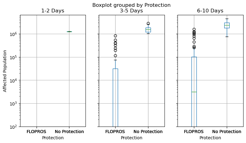
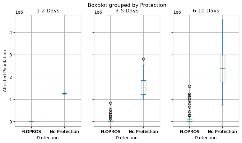
We compute the impacts for all time frames of both series and visualize the resulting distributions with boxplots.

impact_series = pd.Series(
    [
        ImpactCalc(exposure, impf_set_affected, haz).impact(assign_centroids=False)
        for _, haz in hazard_series.items()
    ],
    index=hazard_series.index,
)
impact_series_flopros = pd.Series(
    [
        ImpactCalc(exposure, impf_set_affected, haz).impact(assign_centroids=False)
        for _, haz in hazard_series_flopros.items()
    ],
    index=hazard_series_flopros.index,
)

2024-02-29 15:01:41,831 - climada.engine.impact_calc - INFO - Calculating impact for 2606616 assets (>0) and 50 events.
2024-02-29 15:01:41,991 - climada.engine.impact_calc - INFO - Calculating impact for 2606616 assets (>0) and 50 events.
2024-02-29 15:01:42,161 - climada.engine.impact_calc - INFO - Calculating impact for 2606616 assets (>0) and 50 events.
2024-02-29 15:01:42,339 - climada.engine.impact_calc - INFO - Calculating impact for 2606616 assets (>0) and 50 events.
2024-02-29 15:01:42,434 - climada.engine.impact_calc - INFO - Calculating impact for 2606616 assets (>0) and 50 events.
2024-02-29 15:01:42,541 - climada.engine.impact_calc - INFO - Calculating impact for 2606616 assets (>0) and 50 events.

df_impacts = pd.concat(
    [
        pd.DataFrame.from_records(
            {str_idx: imp.at_event for idx, imp in impact_series.items() for str_idx in idx if isinstance(str_idx, str)}
            | {"Protection": "No Protection"}
        ),
        pd.DataFrame.from_records(
            {str_idx: imp.at_event for idx, imp in impact_series_flopros.items() for str_idx in idx if isinstance(str_idx, str)}
            | {"Protection": "FLOPROS"}
        ),
    ]
)
axes = df_impacts.boxplot(
    column=["1-2 Days", "3-5 Days", "6-10 Days"],
    by="Protection",
    figsize=(9, 4.8),
    layout=(1, 3),
)
axes[0].set_ylabel("Affected Population")

Text(0, 0.5, 'Affected Population')

axes = df_impacts.boxplot(
    column=["1-2 Days", "3-5 Days", "6-10 Days"],
    by="Protection",
    figsize=(9, 4.8),
    layout=(1, 3),
)
axes[0].set_ylabel("Affected Population")
axes[0].set_yscale("log")
axes[0].set_ylim(bottom=1e2)

(100.0, 6561677.47926394)